Bridge-Crossing the Human Genome

At university, taking pure mathematics units can at times feel like an intentional retreat from reality. Here, the world of politics, social enterprises and humanity in general tends to vanish in the limit to be replaced by abstractions, generalisations and shunting Greek symbols around on a whiteboard¹. In many ways, it is this process of entering such a foreign world that is so enticing. But, every now and again, it can be endlessly refreshing to see a tangible application of something that a priori seems to have no bearing on the real world. I would like to present one such example I came across in graph theory a few weeks ago.

Circuits, Cycles, Trails, Walks and Paths

I'm going to assume from here on that you are familiar with the basics of graph theory. However, just to recap ever so briefly, a graph $G$ consists of two things:

1. A vertex set $V(G)$ which you may like to think of as nodes of the graph
2. An edge set $E(G)$, which connects two vertices together. An edge $e\in E(G)$ is generally written as $e=uv$ for two vertices $u,v \in V(G)$.

In the above graph $G$, the vertex set is $V(G)=\{a, b, c, d, e, f\}$ and the edge set is $E(G)=\{ab, ad, ac, bc, bd, cd, de, df, ef\}$

A natural question here is to wonder, for a given graph $G$, whether there exists a way of getting from one vertex to another by edge-traversal for any two vertices you might select. What about a way of getting from $a$ to $f$ in the above that goes through each vertex exactly once? These are, it turns out, entirely non-trivial matters, and I hope only in this piece to explore but one aspect of them. So, let's start with some definitions:

Walk: A finite length alternating sequence of vertices and edges. This is generally written in the form of $a, d, c, f, e, d$ where the edges taken are implied.

Path: A walk in which there are no repeated vertices (and hence no repeated edges)

Trail: A walk in which there are no repeated edges (but which may contain repeated vertices)

Cycle: A closed path, closed here meaning that the path starts and ends at the same vertex

Circuit: A closed trail

Using the above graph as an example:

The two final definitions, and perhaps the most important ones for the purposes of this piece, are the following:

Hamiltonian cycle: A cycle is Hamiltonian if it is a cycle that passes through every vertex. A graph $G$ that contains a Hamiltonian cycle is Hamiltonian.

Eulerian circuit: A circuit is Eulerian if it contains every edge. A graph $G$ that contains an Eulerian circuit is Eulerian.

The definitions of a Hamiltonian path and Eulerian trail are analogous.

The last primer is that we can have what is called a directed graph, in which the edge $e=uv\in E(G)$ actually specifies movement from $u$ to $v$ (not both ways as a normal edge does). This offers a slight restriction or complication of matters when it comes to finding a trail or path in a directed graph.

What we will turn to next are ways (if any) of determining in a non-exhaustive fashion whether a graph is Hamiltonian and/or Eulerian. Obviously, you could throw a brute-force trial of all possible cycles and circuits at the problem, but the number of such possibilities grows exponentially on the number of vertices/edges in the graph. And for the graphs we will be considering by the end, concerning human genomes with millions of base pairs, this is clearly not ideal. So, before proceeding, can you conjure such a characterisation for whether a graph is/isn't Hamiltonian/Eulerian? Take the below graphs as examples.

It turns out that there aren't any strong characterisations of graphs that have Hamiltonian cycles. By a characterisation, we mean a statement of the form "A graph is Hamiltonian if and only if ". Additionally, and more pertinently for this excursion, there is no (currently known) polynomial-time algorithm for determining whether a graph is Hamiltonian. For an $n-$vertex graph you could just as well check all $n!$ permutations of the vertices and see if any reveal a Hamiltonian cycle, but this gets outrageously expensive for large $n$. The accurate statement here is to say that the problem of Hamiltonian finding is NP-complete.

On Algorithmic Complexity (OPTIONAL)

Without getting lost in the weeds, in Computer Science there are classes that we can assign a problem to which give us some measure of the "difficulty" of the problem. The more inner the circle, the "easier" it is to solve. At the outer bounds of this map are problems that are not even solvable in any sort of conventional, computerised/algorithmic fashion. What interests us here are the circles of P and NP (polynomial and non-polynomial). A P type problem is one for which there exists a polynomial-complexity (denoted commonly as $\mathcal{O}(n^c)$ for some constant $c$ where $n$ is the size of the problem input) that solves the problem. An example is finding the largest element in a list of $n$ numbers, since you need only walk over the list one time to find it (precisely, this is a linear time, or $\mathcal{O}(1)$ algorithm).

An NP type problem is one for which no such polynomial-time solver exists, but for which there exists a polynomial-time validator for solutions to the problem. That is, I might not be able to find a Hamiltonian cycle in a graph $G$ efficiently, but if you give me an ordering of the vertices, I can efficiently check whether or not the ordering is a Hamiltonian cycle or not. Last remark here: the "complete" part of NP-complete means that any other NP problem can, in some efficient (read: polynomial time) fashion be translated into this problem of Hamiltonian cycles. This is of interest to computer scientists because there is an open problem $P=NP$ which investigates whether in fact the green and red circles above are in fact one and the same. One approach to solving this is to find some NP-complete problem like Hamiltonian cycles, show that it is in fact a P-type problem, and via the NP-completeness of it conclude that all other NP problems are in fact P.

The final comment for this section is that because finding a Hamiltonian cycle is NP-complete, so too is the problem of finding a Hamiltonian path. This is because a Hamiltonian path is just a Hamiltonian cycle with one edge removed (between the start and end vertices of the path).

End of Tangent

Okay, so the key takeaway here is that the nature of Hamiltonian cycles is complicated. To finish this section, let's list out a few things that we do know about when a graph will be Hamiltonian.

The $n\times n$ grid graph is Hamiltonian if and only if $n$ is even. An example of the grid graph with $n=4$ is shown below. It should be fairly trivial to come up with the Hamiltonian cycle.

There are a few more examples of graphs that we can say are definitely Hamiltonian, but more revealing is the following:

Theorem: Every graph $G$ with $n$ vertices and minimum degree (denoted $\delta(G)$) of at least $n/2$ is Hamiltonian²

This can be easily proved by contradiction, along with this additional lemma:

Lemma: If $u, w$ are adjacent vertices of an $n-$vertex graph $G$ satisfying $\deg(u)+\deg(v)\ge n$ and $G+uw$ (the graph $G$ plus the new edge $uw$) is Hamiltonian, then $G$ is Hamiltonian.

Conclusion - thinking about Hamiltonian paths and cycles is inefficient and we struggle to characterise whether they exist. Let's see if the same is true of Eulerian circuits and trails.

On Bridge Crossings

The punchline: it is not. And it stems from a discovery by arguably the greatest mathematician of all time, Leonhard Euler.

In the early 18th century, the Prussian city of Königsberg, now Kaliningrad (Russia)³, was home to some lovely bridges, and the story goes that its citizens wondered if you could, from a particular starting point, walk a circuit that crossed each bridge exactly once. This should hopefully remind us of Eulerian circuits discussed earlier, and the problem can easily be translated to a graph with each region of the city a vertex, and each bridge an edge (Source: MathsCareers).

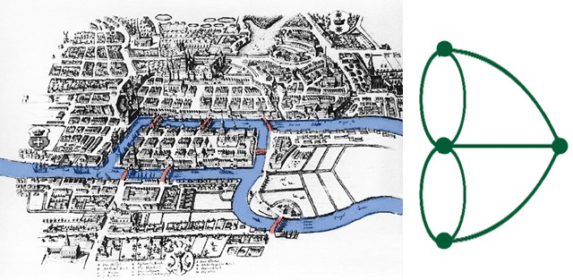
In 1735, Euler proved that there exits no Eulerian circuit for the above graph. This is because unlike Hamiltonian graphs, there is a strong and very simple characterisation of Eulerian graphs.

Theorem: A multigraph is Eulerian if and only if it is connected and every vertex has even degree.

A multigraph is an extension of the definition of a graph where we allow for multiple edges between the same vertices, and connected means that there is a path in the graph between any two vertices.

Proof

Unlike the theorem linking minimum degree to Hamiltonian graphs, the above theorem is an if and only if statement. This effectively whisks two results into one: (1) that if a graph is Eulerian it is connected and every vertex has even degree, and (2) that if a graph is connected with every vertex having even degree, it is Eulerian. These two statements are not the same (the implication is reversed) and so they require two proofs.

For the forward direction, consider an Eulerian multigraph $G$ and one of its vertices, $v$. Every time the circuit visits $v$, it arrives on some edge and then leaves on a different edge. Hence there are always two edges involved with each interaction of $v$, and since each edge is visited precisely once, $\deg(v)$ is even. The only vertex for which this is perhaps not immediately obvious is the start (and hence final) vertex. However, we can pair up the very first and very last edge together and treat the remaining edges in the same way as any another vertex. Since the circuit visits every edge once, it clearly must also visit every vertex at least once. Hence for two vertices $v$ and $w$ we can find a walk between them that is some subsection of the entire circuit. And from this, we can produce a path (remember, no repeated vertices) - think about cutting out all of the loop-bits of the walk. So the graph $G$ is connected and we have proven the forward direction.

For the backward direction, we can simply provide an algorithm that generates an Eulerian circuit from a connected graph with every vertex of even degree. This algorithm is due to Hierholzer:

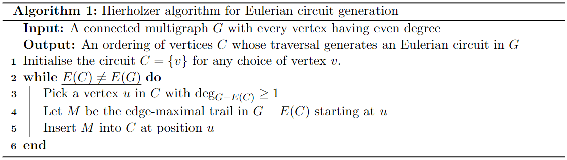
As stated right at the start of this article, walks, paths, circuits, etc. are generally constructed as an ordering of some (or all) of the vertices of a graph. The way to think about this algorithm is that it grows the circuit bit by bit. So to start, Line 1 instructs us to select a particular vertex as our starting point (here, $v$). The condition in the while loop of Line 2 is translated as being "there are still edges in the original graph not included in our current circuit $C$ - of course a requirement, given that an Eulerian circuit has to include all of the graph edges. Line 3 says to find a vertex $u$ in the current circuit whose degree in the graph constructed by taking $G$ and removing all of the edges currently contained in the circuit is at least one. Such a vertex must always exist as $G$ is connected. If not, then we would have some vertex that is unreachable from the growing circuit, i.e. $G$ is in fact not connected. Next we construct the largest possible trail (a walk in which there are no repeated edges (but which may contain repeated vertices)) $M$ judged by the number of edges it contains which starts at $u$. The kicker here is that this trail must also finish at $u$ because every vertex has even degree, for reasons highlighted in the proof of the forward direction. We now grow the circuit $C$ by inserting this partial circuit $M$ into it at $u$⁴.

The last observation before moving onto the interesting stuff is that this characterisation can be modified (ever so slightly) to establish when a graph has an Eulerian trail (using all the edges but not finishing at the same vertex). Since an Eulerian circuit can be made from a trail by adding an edge between the start and end vertex, removing an edge from an Eulerian graph will mean it has an Eulerian trail. Since every vertex start with even degree, and we removed one edge, the following characterisation of graphs with Eulerian trails follows naturally:

Theorem: A multigraph has an Eulerian trail if and only it is connected and exactly two vertices have odd degree (the rest having even degree).

The start and end vertices of the trail must be the two vertices with odd degree.

A Graph Theorist and a Biologist Walk Into a Bar

With all that out of the way, it's time to get to the lovely application of Eulerian circuits and paths to real-world problems. Here, I wish to highlight just one.

The Human Genome Project (beginning 1984) set out to write the entire sequence of base pairs in human DNA. As a refresher, there are four bases (adenine (A), cytosine (C), guanine (G) and thymine (T)) known as nucleotides whose ordering encodes for the information available in creating and maintaining an organism. Up to a remarkably high percentage, all human DNA consists of the same base sequences. Human DNA has a length of about 3 billion base pairs. In the early 2000s as the first drafts were being completed of the human genome, DNA sequencers were a developing technology. At a high level, these machines take a long DNA strand and split into small fragments (known as reads) which it can identify the base sequencing of. There are two issues, though, The reads with the best sequencers only get up to around 1000 base pairs, and so how then can we reconstruct the full sequence from a collection of reads?

Problem Description

Given a set of DNA fragments $\mathcal{F}$, reconstruct the original sequence $\mathcal{S}$. In this process, we will make two assumptions (which in reality are not needed, and can be overcome, but for our discussion will make matters more lucid):

Every fragment in $\mathcal{F}$ has the same length $\ell$

$\mathcal{F}$ contains all possible fragments of length $\ell$ from the original sequence $\mathcal{S}$. By way of example, if $\mathcal{S}=ACGTAGGA$ and $\ell=3$, then we would have $\mathcal{F}=(ACG, CGT, GTA, TAG, AGG, GGA)$.

The Hamiltonian Approach

Like the Königsberg problem, we first wish to translate this problem into a graph. The most immediate choice is to make each fragment in $\mathcal{F}$ a vertex. For the edges, the "natural" selection is to have an edge between two vertices (read fragments) whenever they are identical up to the first and last bases. That is, given two fragments $u=u_1,u_2,\ldots,u_\ell$ and $v=v_1,v_2,\ldots,v_\ell$, we have an edge between $u$ and $v$ if $u_1,u_2,\ldots u_{\ell-1}=v_2,v_3,\ldots,v_\ell$. So if $\ell=5$ and we have fragments $f_1=A\underline{AGTC}, f_2=\underline{AGTC}C, f_3=GCATT$, we would have an edge between $f_1$ and $f_2$ but no edge from $f_3$ to either $f_1$ or $f_2$.

So, due to the second assumption above, given a particular fragment $f_i$, the very next base in the original sequence $\mathcal{S}$ ^^has to come from a fragment $f_{j}$ that is adjacent to $f_i$^^. Using the above example, since $f_2, f_1$ are adjacent, we would extend $f_1$ to a length of 6 by using the final $C$ of $f_2$, yielding $AAGTCC$.

Convince yourself then that $\mathcal{S}$ must be reconstructed by a Hamiltonian path of the fragment graph. But remember, from earlier discussion, that there is no efficient algorithm for producing a Hamiltonian path in a graph, even if we knew (somehow) that it had one. Because generating a Hamiltonian path is non-polynomial, at the scale of billions of base pairs, this process of sequence reconstruction would take huge amounts of time and compute. So we need an alternative.

The Eulerian Approach

Pevzner, Tang, & Waterman (2001) proposed an alternative solution that solves the reconstruction dilemma in polynomial time. To do this, we need to alter the translation of fragments into the graph, effectively reversing the role of edges and vertices. Given $\mathcal{F}$ and $\ell$, the insight here is to have as vertices all $\ell-1$ fragments taken from $\mathcal{F}$. So if $\mathcal{F}=(ACG, CGT, GTA, TAG, AGG, GGA)$ as before, then the vertices of our graph $G$ would be $V(G)=\{AC, CG, GT, TA, AG, GG, GA\}$. Note that this process should ignore an $\ell-1$ fragment if it is already present as a vertex. Then the edges of the graph correspond fragments in $\mathcal{F}$. In particular, for each fragment $f=f_1,f_2,\ldots, f_\ell$ there will be an edge from $f_1,f_2,\ldots, f_{\ell-1}$ to $f_2,f_3,\ldots, f_\ell$.

The beauty is that now, the reconstruction of $\mathcal{S}$ corresponds to an Eulerian trail of $G$, which we know can be found very efficiently indeed. Elegant!

Concretising With an Example

Let's consider an example comparing both approaches. In both, we will consider the set of reads $\mathcal{F}=ATG, TGG, TGC, GTG, CGT, GCG, GGC, GCA$. With the Hamiltonian approach, our graph would look as follows:

But with the Eulerian approach detailed by Pevzner et. al:

The above graph does indeed have an Eulerian trail as it satisfies the characterisation theorem outlined earlier (only $AT, CA$ have odd degree). An Eulerian trail is given by:

$AT, TG, GG, GC, CG, GT, TG, GC, CA$

which produces the sequence $\mathcal{S}=ATGGCGTGCA$.

The keen eye may note another Eulerian trail above, namely $AT, TG, GC, CG, GT, TG, GG, GC, CA$, which yields $\mathcal{S}=ATGCGTGGCA$. This, among some other issues, is one of the problems with our simplified model. In practice, these can be overcome but this lies outside the scope of what I wish to cover. Suffice to say, though, this approach implemented within the context of the HGP exponentially reduced the complexity of sequence reconstruction.

References

Pevzner, P. A., Tang, H., & Waterman, M. S. (2001). A new approach to fragment assembly in DNA sequencing. Proceedings of the Fifth Annual International Conference on Computational Biology, 256–267.

Footnotes